Chapter 3 Analyze the effect of UDCA administration on the bile acid pool (supplementary figure 5)
#summarize bile acid pools
both_conc<- cohort_BAS %>% select(-ursodiol)%>%
  left_join(conc_all_filtered) %>% clean_names()

#prep dataset prepping each BA depending on its classifications
both_conc_pools<-both_conc %>%
  gather("bile_acid", "value", names(.)[8]:names(.)[ncol(.)]) %>%
  select(-gi_gvhd, -later, -periengr) %>%
  filter(bile_acid!="beta_muricholic_acid") %>% #removing because it's not measured in all samples
  filter(bile_acid!="omega_muricholic_acid") %>%  #removing because it's not measured in all samples
  categorize_bile_acids(ba_families)

both_conc_pools_final<-both_conc_pools %>%
  group_by(sampleid) %>%
  summarise(across(where(is.numeric), sum)) %>%
  left_join(ursodiol)

#rearrange ursodiol
both_conc_pools_final$ursodiol <-factor(both_conc_pools_final$ursodiol,
                           levels=c("Y","2-3w","3-4w","1-2m", "N"))
##Evaluation of ursodiol exposure and UDCA concentration
ursodiol_BAs<-both_conc %>%
  left_join(ursodiol)

#rearrange ursodiol
ursodiol_BAs$ursodiol <-factor(ursodiol_BAs$ursodiol,
                           levels=c("Y","2-3w","3-4w","1-2m", "N"))

ursodiol_BAs %>%
  ggplot(aes(x=ursodiol, y=log10(`ursodeoxycholic_acid`), color=ursodiol)) +
  geom_boxplot(width=0.2, outlier.shape =NA, lwd=.7)+
  geom_jitter(width=0.2, alpha=0.2)+
  theme_classic() +
  xlab("ursodiol exposure")+
  stat_compare_means(comparisons=list( c("Y", "2-3w"),c("3-4w", "Y"), c("Y", "1-2m"), c("N", "Y"),
                                       c("3-4w", "2-3w"),c("1-2m", "2-3w"), c("N", "2-3w"),
                                       c("1-2m", "3-4w"),  c("N", "3-4w"),
                                       c("N", "1-2m")
  ),
  #label="p.signif",
  method="wilcox.test",
  correct=FALSE)+
  scale_color_manual(values=c("#a6611a", "#bf812d","#dfc27d", "#80cdc1", "#018571"))+
  theme(legend.position="none")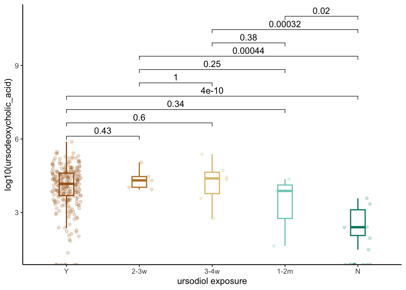
3.1 Plot ursodiol exposure and secondary BAs concentrations
both_conc_pools_final %>%
  ggplot(aes(x=ursodiol, y=log10(secondary_pool), color=ursodiol)) +
  geom_boxplot(width=0.2, outlier.shape =NA, lwd=.7)+
  geom_jitter(width=0.2, alpha=0.2)+
  theme_classic() +
  xlab("ursodiol exposure")+
  stat_compare_means(comparisons=list( c("Y", "2-3w"),c("3-4w", "Y"), c("Y", "1-2m"), c("N", "Y"),
                                       c("3-4w", "2-3w"),c("1-2m", "2-3w"), c("N", "2-3w"),
                                       c("1-2m", "3-4w"),  c("N", "3-4w"),
                                       c("N", "1-2m")
  ),
  #label="p.signif",
  method="wilcox.test",
  correct=FALSE)+
  scale_color_manual(values=c("#a6611a", "#bf812d","#dfc27d", "#80cdc1", "#018571"))+
  theme(legend.position="none")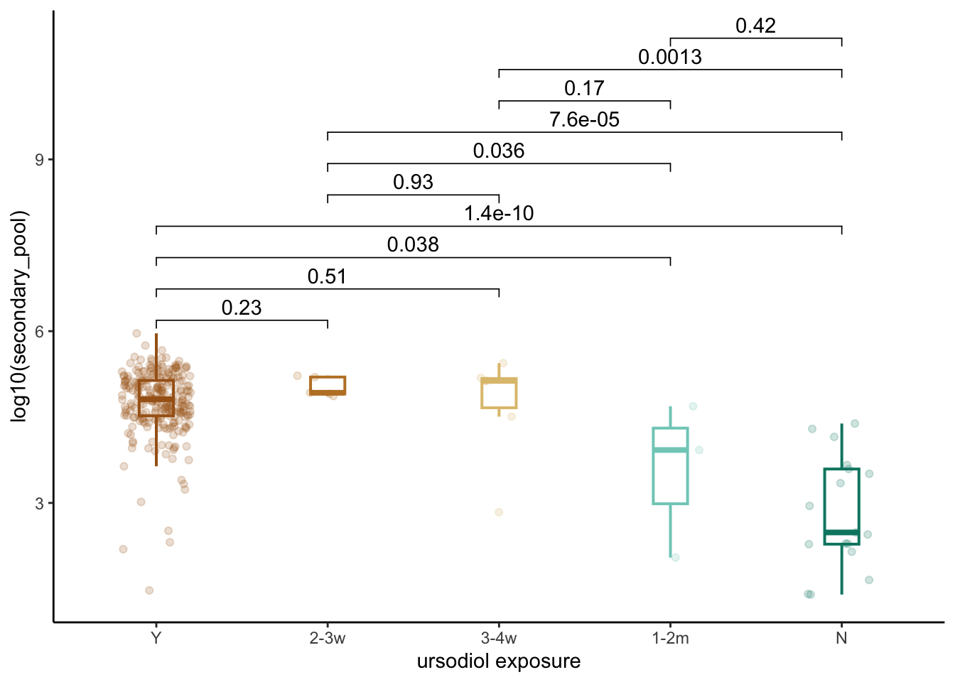
3.2 Plot correlation of ursodiol with other bile acid pools: plot conjugated UDCA (tauroursodeoxycholic_acid+glycoursodeoxycholic_acid), TBAs (total_BAs), PBAs (primary_pool), SBAs (secondary_pool), nonUDCA total BAs (total_nonUDCA_pool), nonUDCA SBAs (secondary_nonUDCA), secondary/primary ratio (SP_ratio)
both_conc_pools_final %>%
  mutate(SP_ratio=secondary_pool/primary_pool) %>%
  mutate(SP_ratio_nonUDCA=secondary_nonUDCA/primary_pool) %>%
  left_join(both_conc %>% select(sampleid, glycoursodeoxycholic_acid, tauroursodeoxycholic_acid, ursodeoxycholic_acid)) %>%
  ggplot(aes(y=log10(`ursodeoxycholic_acid`+2.5), x=log10(secondary_pool+2.5)))+
  geom_point(size=0.8, alpha=0.4)+
  geom_smooth(method="lm")+
  stat_cor(method = "pearson")+
  #ylab("log10(UDCA)")+
  #xlab("log10(PS_nonUDCA)")+
  theme_classic()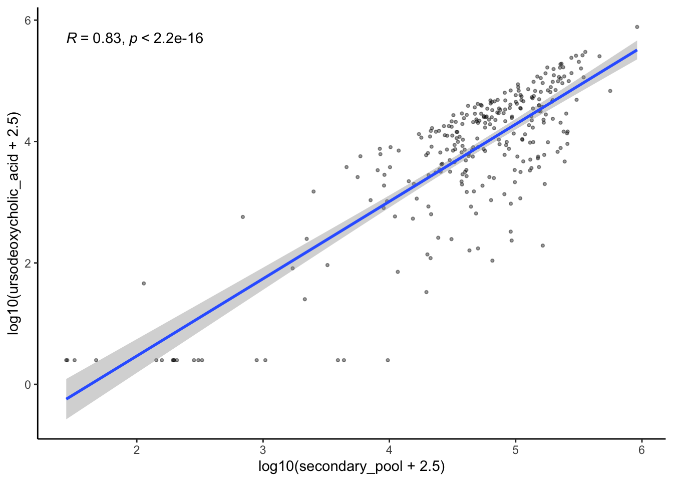
3.3 Create correlation plots to evaluate association of UDCA with all individual BAs
library(corrplot)

precor_data<- filtered_combined_table %>%
  column_to_rownames("sampleid")
cor_data<-cor(precor_data, use = "complete.obs")

corrplot(cor_data)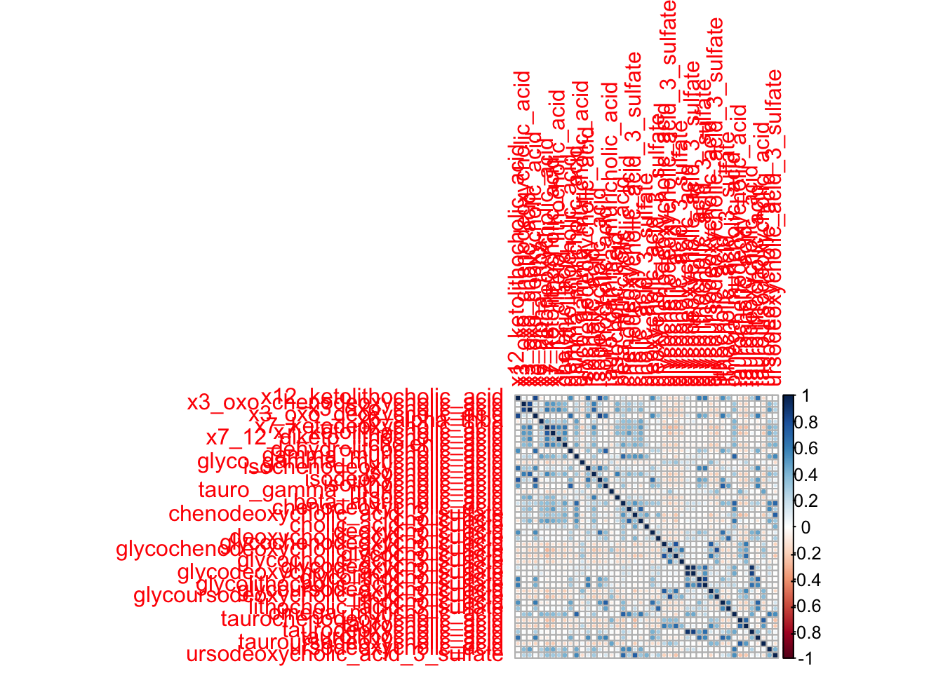
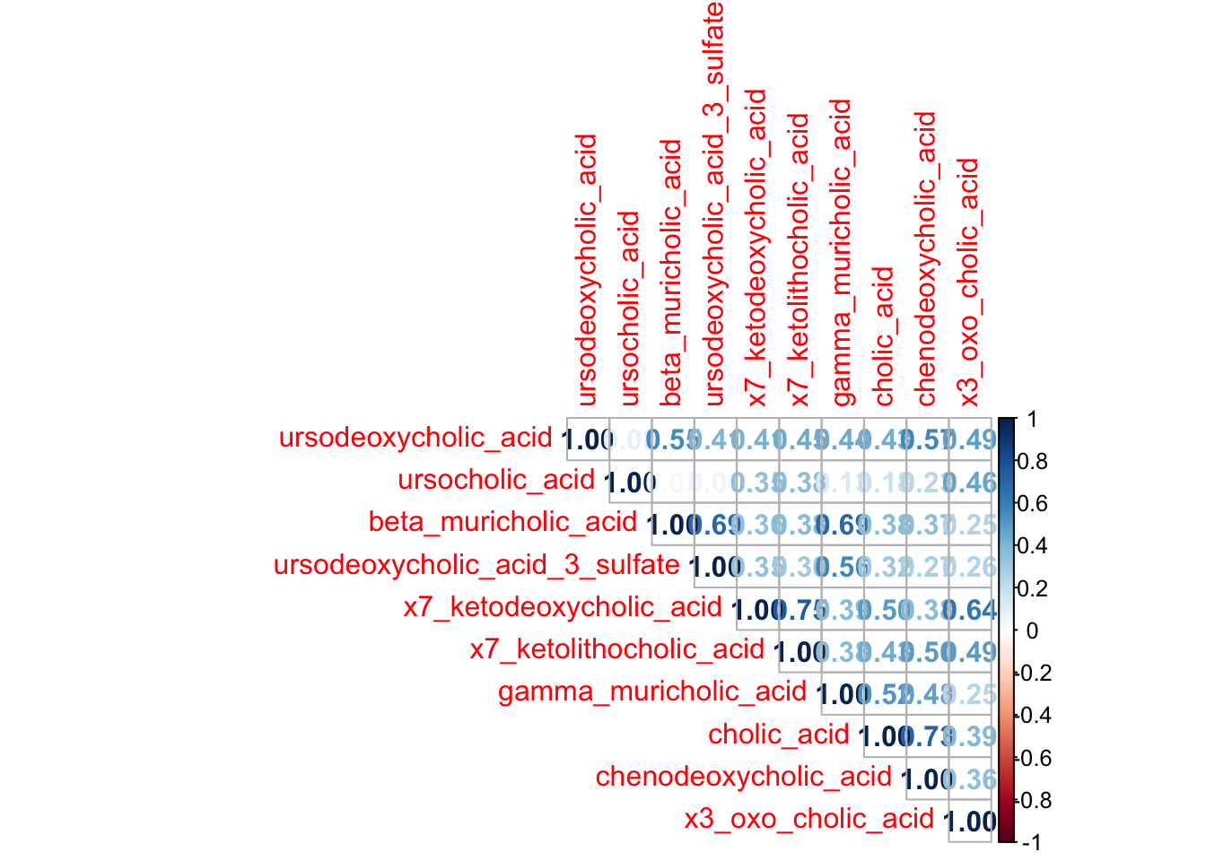
3.3.1 Visualization of significant correlations of UDCA with individual BAs (R>0.4)
precor_data_selected<- filtered_combined_table %>%
  column_to_rownames("sampleid") %>%
  select(ursodeoxycholic_acid, ursocholic_acid, beta_muricholic_acid, ursodeoxycholic_acid_3_sulfate, x7_ketodeoxycholic_acid,
         x7_ketolithocholic_acid, gamma_muricholic_acid, cholic_acid, chenodeoxycholic_acid, x3_oxo_cholic_acid)

cor_data_selected<-cor(precor_data_selected, use = "complete.obs")

corrplot(cor_data_selected, method = "number", type = "upper")