Chapter 6 Shotgun metagenomic sequencing: Evaluate genes of interest (figure 5, supplement figure 10)
6.1 BSH
6.1.1 Evaluate BSH abundance at peri-GVHD onset
BSH_metalphlan %>%
  left_join(cohort_BAS) %>%
  filter(later=="Y") %>%
  ggplot(aes(x=GI_GVHD, y=log10(cpm+0.55), color=GI_GVHD))+
  geom_boxplot(width=0.2, lwd=0.8, outlier.shape = NA) +
  geom_jitter(width=0.3, alpha=0.3, size=2.5)+
  ylab("log10(BSH)")+
  xlab("")+
  theme_classic()+
  stat_compare_means(comparisons=list(c("Y", "N")),
                     method="wilcox.test",
                     correct=FALSE)+
  scale_color_manual(values=c("dodgerblue4", "red3"))+
  theme(legend.position="none")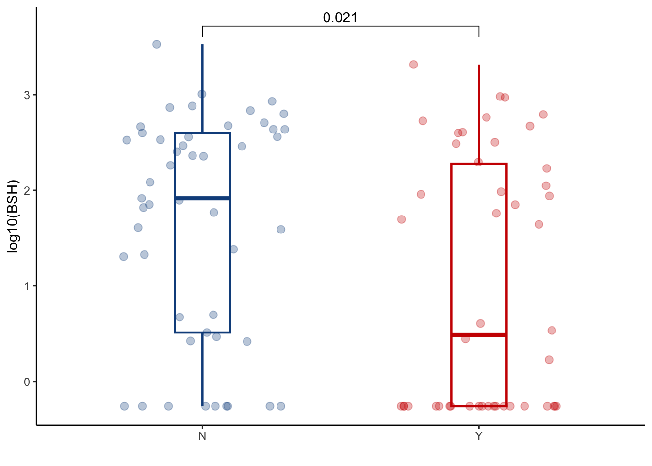
6.1.2 Evaluate BSH abundance at peri-engraftment time point
BSH_metalphlan %>%
  left_join(cohort_BAS) %>%
  filter(periengr=="Y") %>%
  ggplot(aes(x=GI_GVHD, y=log10(cpm+0.05), color=GI_GVHD))+
  geom_boxplot(width=0.2, lwd=0.8, outlier.shape = NA) +
  geom_jitter(width=0.3, alpha=0.3, size=2.5)+
  ylab("log10(BSH)")+
  xlab("")+
  theme_classic()+
  stat_compare_means(comparisons=list(c("Y", "N")),
                     method="wilcox.test",
                     correct=FALSE)+
  scale_color_manual(values=c("dodgerblue4", "red3"))+
  theme(legend.position="none")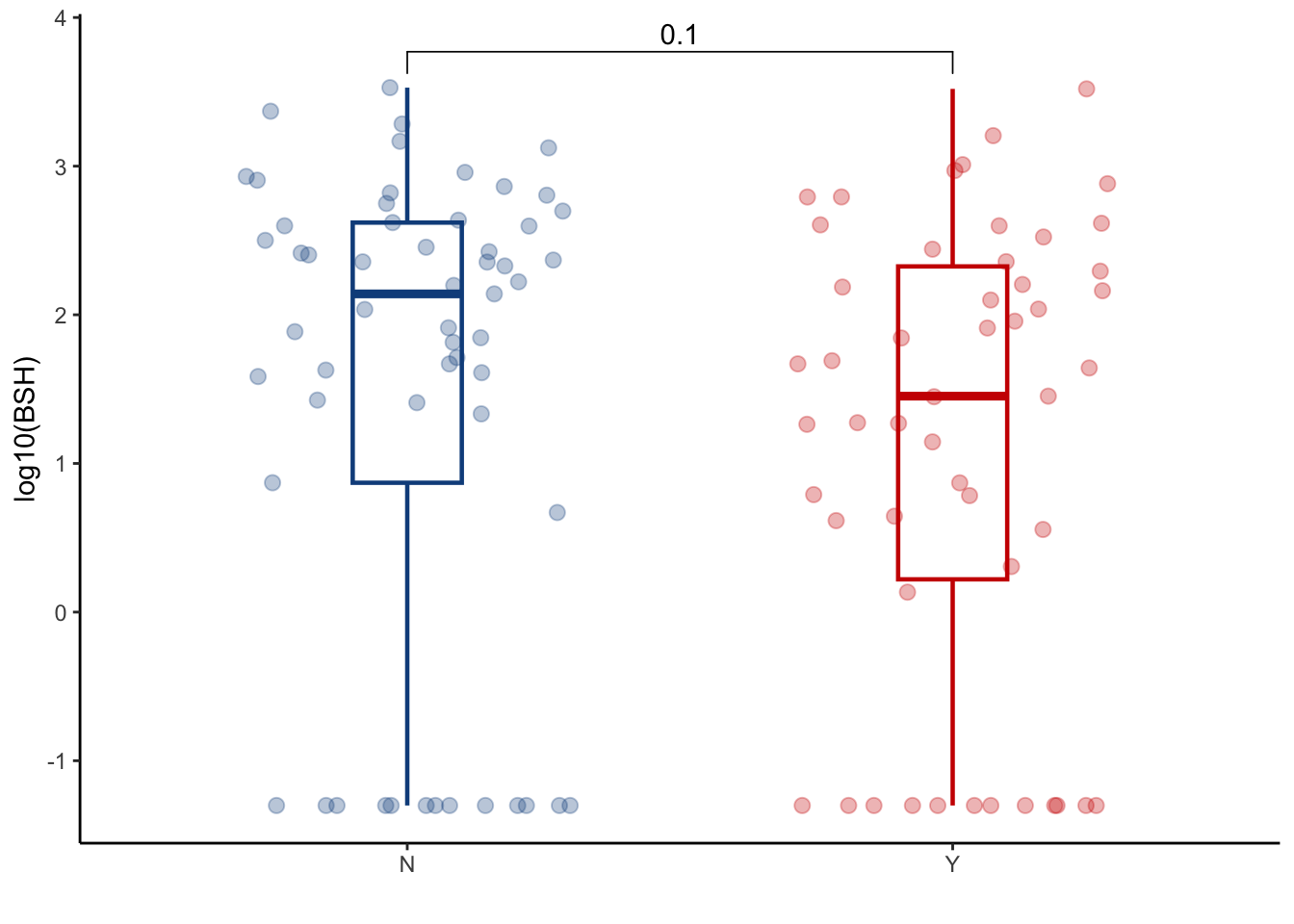
6.2 Bai operon gene
6.2.1 Evaluate correlation of bai operon gene sum and nonUDCA secondary BAs
bai_genes_clean %>%
  distinct(sampleid, bai_operon_sum ) %>%
  inner_join(both_conc_pools_final) %>%
  ggplot(aes(x=log(secondary_nonUDCA), y=log(bai_operon_sum+0.05)))+
  geom_point(alpha=0.6)+
  stat_cor(method="pearson")+
  geom_smooth(method="lm")+
  theme_classic()+
  ylab("bai operon log10(cpm)")+
  xlab("SBAs* log10(pmol/mg)")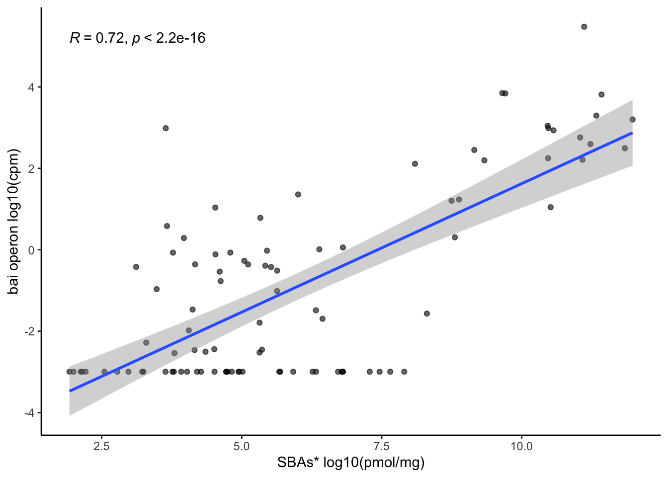
6.2.2 Bai operon gene sum in peri-GVHD onset
bai_genes_clean %>%
  distinct(sampleid, bai_operon_sum ) %>%
  inner_join(cohort_BAS %>% select(sampleid, GI_GVHD, later, ursodiol) %>% filter(later=="Y")) %>%
  ggplot(aes(x=GI_GVHD, y=log(bai_operon_sum+0.01), color=GI_GVHD))+
  geom_boxplot(width=0.2, lwd=0.8, outlier.shape = NA) +
  geom_jitter(width=0.3, alpha=0.3, size=2.5) +
  ylab("log10(bai_operon_sum)") +
  xlab("") +
  theme_classic() +
  stat_compare_means(comparisons=list(c("Y", "N")),
                     method="wilcox.test",
                     correct=FALSE)+
  scale_color_manual(values=c("dodgerblue4", "red3")) +
  theme(legend.position="none")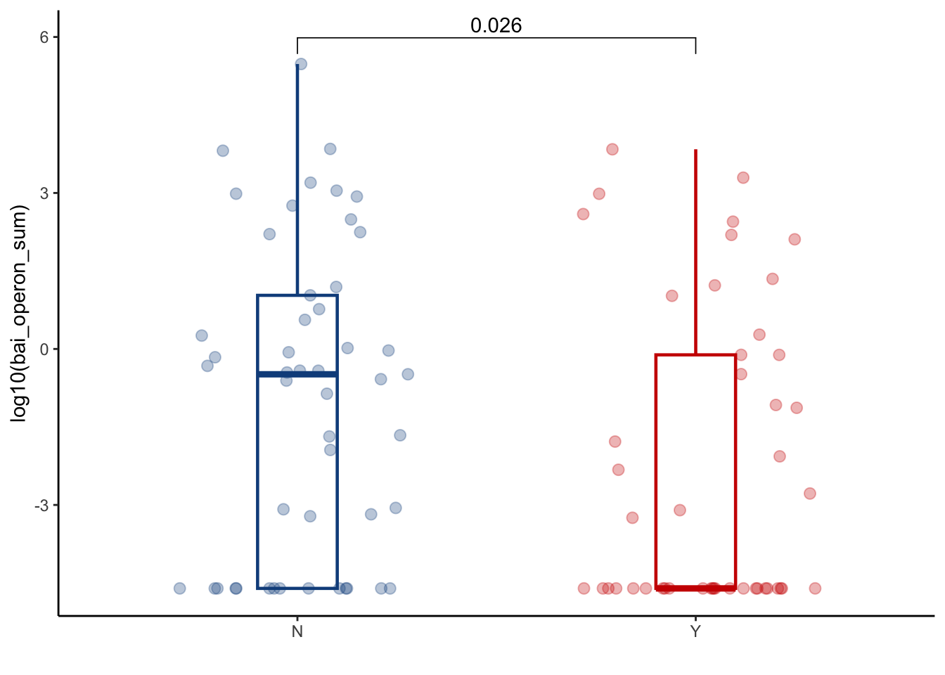
6.2.3 Bai operon individual gene abundance
bai_genes_clean %>%
  inner_join(cohort_BAS %>% select(sampleid, GI_GVHD, later) %>% filter(later=="Y")) %>%
  ggplot(aes(x=GI_GVHD, y=log(cpm+0.01), color=GI_GVHD))+
  geom_boxplot(width=0.2, lwd=0.8, outlier.shape = NA) +
  geom_jitter(width=0.3, alpha=0.3, size=2.5)+
  ylab("log10(cpm)")+
  xlab("")+
  theme_classic()+
  stat_compare_means(comparisons=list(c("Y", "N")),
                     method="wilcox.test",
                     correct=FALSE)+
  scale_color_manual(values=c("dodgerblue4", "red3"))+
  theme(legend.position="none")+
  facet_grid(.~gene)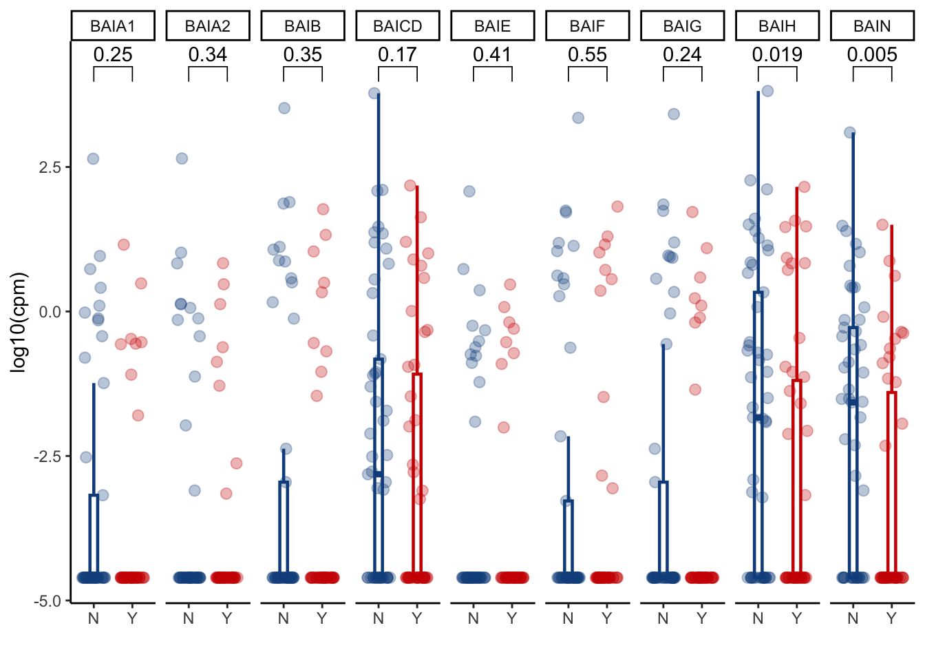
6.3 Bile acid related bacteria
6.3.1 Eggerthella lenta
taxa_bas_later %>%
  ggplot(aes(x=GI_GVHD, y=log10(eggerthella_lenta+ 1.5e-08), color=GI_GVHD))+
  geom_boxplot(width=0.2, lwd=0.8, outlier.shape = NA) +
  geom_jitter(width=0.3, alpha=0.3, size=2.5)+
  ylab("log10(Eggerthella lenta)")+
  xlab("")+
  theme_classic()+
  stat_compare_means(comparisons=list(c("N", "Y")),
                     method="wilcox.test",
                     correct=FALSE)+
  scale_color_manual(values=c("dodgerblue4", "red3"))+
  theme(legend.position="none")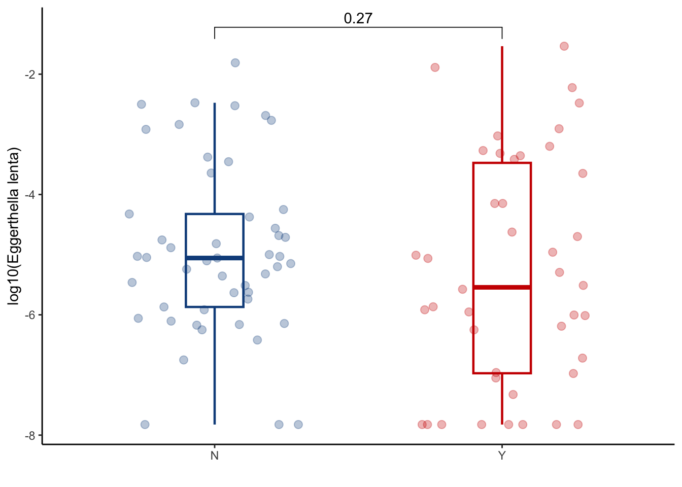
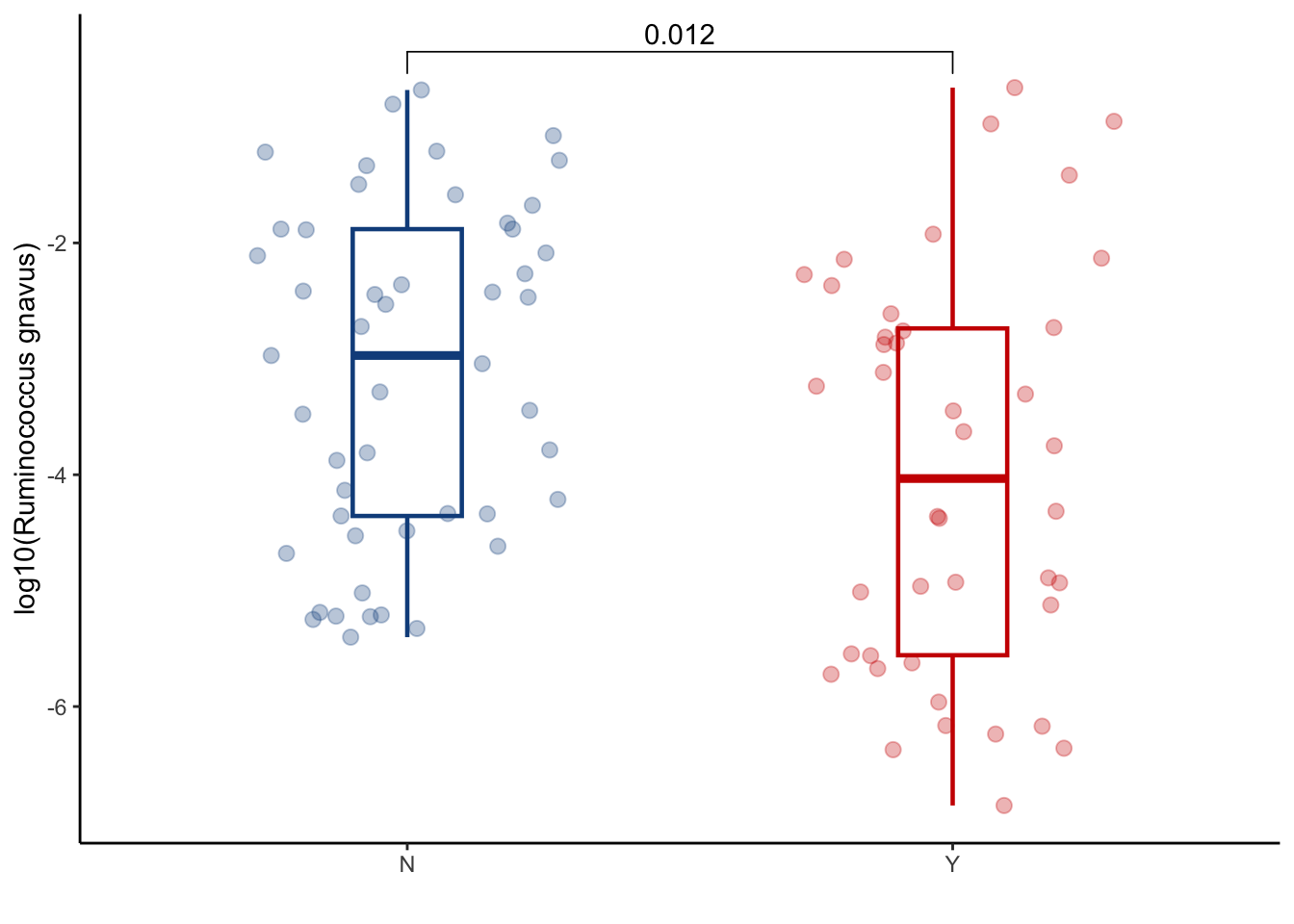
6.3.2 Ruminococcus gnavus
taxa_bas_later %>%
  ggplot(aes(x=GI_GVHD, y=log10(ruminococcus_gnavus+ 1.4e-07), color=GI_GVHD))+
  geom_boxplot(width=0.2, lwd=0.8, outlier.shape = NA) +
  geom_jitter(width=0.3, alpha=0.3, size=2.5)+
  ylab("log10(Ruminococcus gnavus)")+
  xlab("")+
  theme_classic()+
  stat_compare_means(comparisons=list(c("N", "Y")),
                     method="wilcox.test",
                     correct=FALSE)+
  scale_color_manual(values=c("dodgerblue4", "red3"))+
  theme(legend.position="none")