Chapter 11 RNA sequncing in mice (Figure 2): Anastasia Kousa

#renv::activate()
#renv::init()
#renv::install("renv")
#renv::status()
#renv::snapshot()
#renv::restore()

#if (!requireNamespace("BiocManager", quietly = TRUE))
#  install.packages("BiocManager")
#renv::install("bioc::BiocManager", force=T)

#renv::install("bioc::biomaRt", force=T)
#renv::install("bioc::edgeR", force=T)
#renv::install("bioc::EnhancedVolcano", force=T)
#renv::install("tibble", force=T)
#renv::install("ggpubr", force=T)
#renv::install("pheatmap", force=T)
#renv::install("dichromat", force=T)
#renv::install("grid", force=T)
#renv::install("patchwork", force=T)

library(biomaRt)
library(edgeR)
library(EnhancedVolcano)

## Loading required package: ggrepel

library(tibble)
library(ggpubr)
library(pheatmap)
library(dichromat)
library(grid)
library(patchwork)
library(BiocManager)
library(cowplot)

ensembl = useMart(biomart="ENSEMBL_MART_ENSEMBL", dataset="mmusculus_gene_ensembl", host = 'https://may2021.archive.ensembl.org', verbose = TRUE)

## BioMartServer running BioMart version: 0.7
## Mart virtual schema: default
## Mart host: https://may2021.archive.ensembl.org:443/biomart/martservice

## Checking attributes ...Attempting web service request:
## https://may2021.archive.ensembl.org:443/biomart/martservice?type=attributes&dataset=mmusculus_gene_ensembl&requestid=biomaRt&mart=ENSEMBL_MART_ENSEMBL&virtualSchema=default
##  ok
## Checking filters ...Attempting web service request:
## https://may2021.archive.ensembl.org:443/biomart/martservice?type=filters&dataset=mmusculus_gene_ensembl&requestid=biomaRt&mart=ENSEMBL_MART_ENSEMBL&virtualSchema=default
##  ok

11.1 read in file

BMT_liv_int <- read.table( "/Volumes/Macintosh HD/Users/miltiado/Documents/BA/Anastasia/gsea_mice/BMT7_liver-intestine.txt", sep="\t",  row.names=1, header=TRUE, as.is = TRUE, stringsAsFactors = TRUE)
nrow(BMT_liv_int) # needs to be 53379 for GRCm39 -Ensembl 104 May 2021 http://may2021.archive.ensembl.org 104-

## [1] 53379

colnames(BMT_liv_int) <- sub("\\.\\.", '',  sub('_IGO.*', '', colnames(BMT_liv_int)))
rownames(BMT_liv_int) <- sub('\\..*', '', rownames(BMT_liv_int))

11.2 link ensembl ids to gene names

geneNames <- getBM(filters= "ensembl_gene_id", attributes= c("ensembl_gene_id", "external_gene_name"), values=rownames(BMT_liv_int), mart=ensembl)
names <- geneNames[,1]
geneNames <- as.data.frame(geneNames)         
rownames(geneNames) = names
merged <- merge(BMT_liv_int, geneNames, by="row.names", all=FALSE)
BMT_liv_int <- merged[,c(2:24,26)]
rownames(BMT_liv_int) <- merged[,1]

11.3 Read in the count file: - D7

dgeBMT_liv_int <- DGEList(counts=BMT_liv_int[,6:23], genes = BMT_liv_int[,c(24,5)])
rownames(dgeBMT_liv_int$samples)

##  [1] "D7_SI_BM_005"   "D7_LI_BM_002"   "D7_SI_BMT_009"  "D7_SI_BM_004"  
##  [5] "D7_SI_BMT_010"  "D7_LI_BMT_010"  "D7_LIV_BM_004"  "D7_LIV_BM_002" 
##  [9] "D7_LI_BM_005"   "D7_LI_BM_004"   "D7_LIV_BMT_010" "D7_LI_BMT_006" 
## [13] "D7_LIV_BM_005"  "D7_LIV_BMT_009" "D7_LI_BMT_009"  "D7_SI_BM_002"  
## [17] "D7_LIV_BMT_006" "D7_SI_BMT_006"

nrow(dgeBMT_liv_int) # 49915

## [1] 49915

# filter out lowly expressed genes
# count the number of genes that are not expressed in any of the samples - for now subselect only day 7 data: FALSE 32751 TRUE 17164 

table(rowSums(dgeBMT_liv_int$counts==0)==length(rownames(dgeBMT_liv_int$samples))) # FALSE 30678 TRUE 19237

## 
## FALSE  TRUE 
## 30678 19237

dgeBMT_liv_int$condition <- as.factor(sub( '.*_', '',  sub("_0.*", '',  rownames(dgeBMT_liv_int$samples))))
dgeBMT_liv_int$tissue <-  as.factor(sub( '.*_', '',  sub("_B.*", '',  rownames(dgeBMT_liv_int$samples))))
dgeBMT_liv_int$groups <- as.factor(paste0(sub( '_0.*', '', sub('D.?.?_', '', rownames(dgeBMT_liv_int$samples))),"", dgeBMT_liv_int$day))

# filter out lowly expressed genes with filterByExpr function
keep.exprs <- filterByExpr(dgeBMT_liv_int, group=dgeBMT_liv_int$groups)
dgeBMT_liv_int <- dgeBMT_liv_int[keep.exprs,, keep.lib.sizes=FALSE]
# the filtered DGEList-object keeps the gene information for the retained genes correctly associated.
dim(dgeBMT_liv_int) # 17187    18

## [1] 17187    18

# calculate different library sizes
dgeBMT_liv_int <- calcNormFactors(dgeBMT_liv_int)

# create the design model that fits the data, Batch?
designBMT_liv_int <- model.matrix(~0 + dgeBMT_liv_int$groups)
colnames(designBMT_liv_int) <- sub("dgeBMT_liv_int\\$groups", "", colnames(designBMT_liv_int))

# run voom
v <- voom(dgeBMT_liv_int, designBMT_liv_int, plot=TRUE)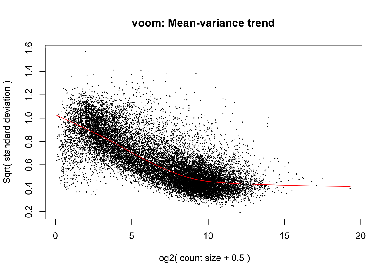

# fit linear model
fit <- lmFit(v, designBMT_liv_int)

cm <- makeContrasts( LI_BMT-LI_BM, 
                     SI_BMT-SI_BM,
                     LIV_BMT-LIV_BM, levels=designBMT_liv_int)

# differential expression analysis
fit2 <- contrasts.fit(fit, cm)
fit2 <- eBayes(fit2)
fit2$groupMeans <- fit$coefficients


x=1
vs = c("LI_BMTvsBM", "SI_BMTvsBM", "LIV_BMTvsBM")

for (x in 1:3) {
  
  BMT_liv_intTable <- topTable(fit2, coef = x, genelist =data.frame(fit2$genes,fit2$groupMeans), number = Inf, adjust="BH")
 # write.table(BMT_liv_intTable, paste0("~/results/v2/", vs[x], "_only_D7.txt"), sep="\t", col.names=NA)
  # save as .rnk for running pathway enrichment analysis with GSEA
  topTable_to_rank <- BMT_liv_intTable
  
# just using logFC as the ranking parameter - or now subselect only day 7 data: c(1,15)
  rankfile = na.omit(topTable_to_rank[,c(1,9)])
  rankfile_sorted = rankfile[order(rankfile$logFC, decreasing = TRUE),]
  #ss  write.table(rankfile_sorted, paste0("/results/v2/", vs[x], "_only_D7.rnk"), sep = '\t', row.names = FALSE, quote = FALSE)
}

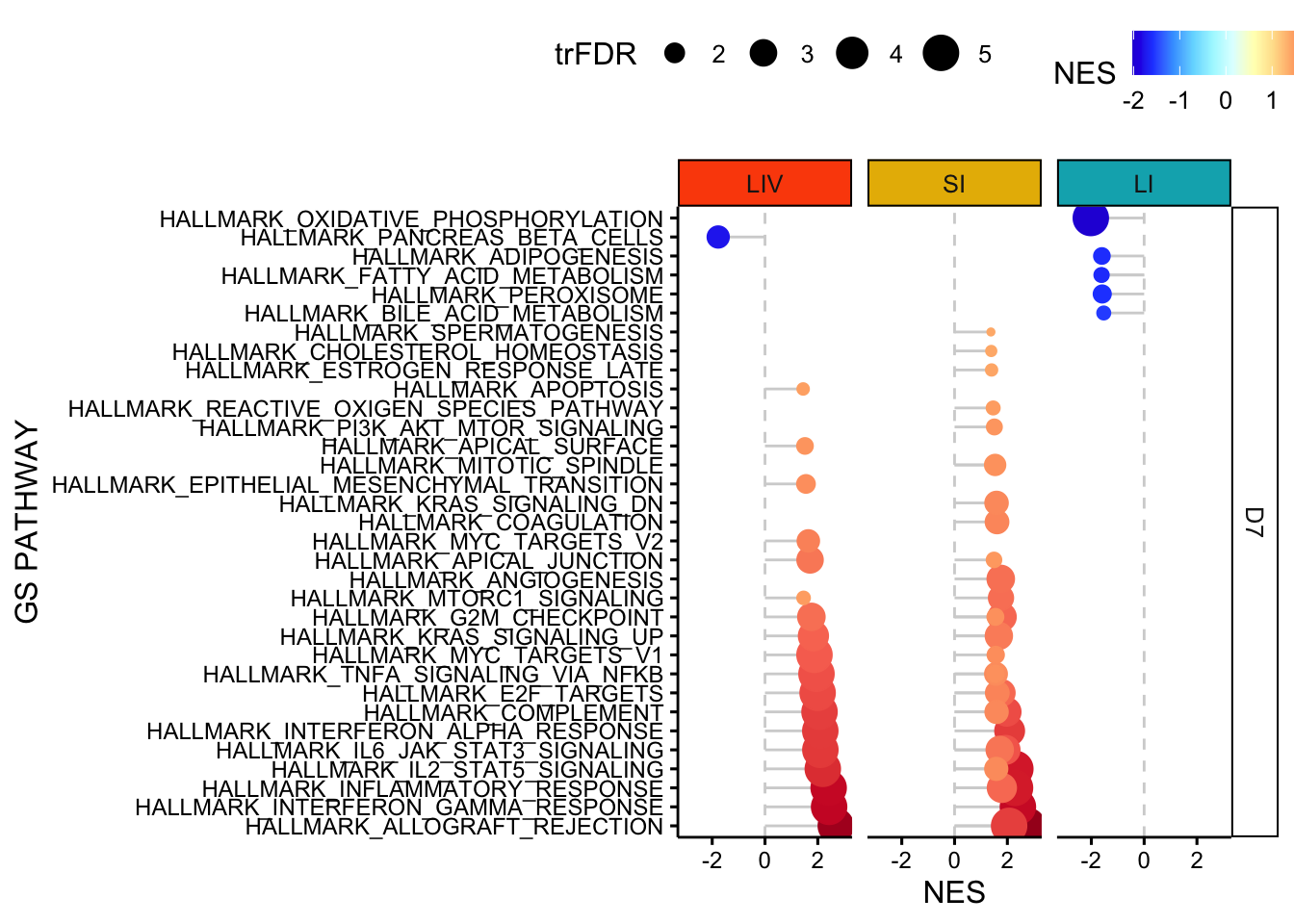
11.4 plot GSEA results facet by organ - Hallmarks - D7

setwd("/Users/miltiado/Documents/BA/Anastasia/gsea_mice/")
gsea_result_files <- list.files(recursive = TRUE, pattern = "^gsea_report(.*)tsv$")
# within the for loop I change the order of the organs
organ_annotation = c("LIV", "LIV", "SI", "SI", "LI", "LI")
day_annotation = c("D7", "D7", "D7", "D7", "D7", "D7")

i=1
all_gsea_results = tibble("GS PATHWAY"=factor(), "GS DETAILS"=integer(), "SIZE"=double(), "ES"=double(), "NES"=double(), "NOM p-val"=double(), "FDR q-val"=double(), "FWER p-val"=double(), "RANK"=integer(), "LEADING EDGE"=factor(), "GROUP"=factor(), "ORGAN" = factor(), "DAY" = factor())

for (path in gsea_result_files[c(3:4, 5:6, 1:2)]){
  gsea_results = tibble(read.table(path, sep="\t", row.names = 1, skip = 1))
  colnames(gsea_results) = c("GS PATHWAY", "GS DETAILS", "SIZE", "ES", "NES", "NOM p-val", "FDR q-val", "FWER p-val", "RANK", "LEADING EDGE", "GROUP")
  gsea_results$GROUP = rep(as.factor(substring(path, 64,76)), nrow(gsea_results))
  gsea_results$ORGAN = rep(as.factor(organ_annotation[i]), nrow(gsea_results))
  gsea_results$DAY = rep(as.factor(day_annotation[i]), nrow(gsea_results))
  all_gsea_results = rbind(all_gsea_results, gsea_results)
  i=i+1
}


all_gsea_results = all_gsea_results[all_gsea_results$NES!="---",]
all_gsea_results$NES = as.double(all_gsea_results$NES)

all_gsea_results$`-10log(FDR q-val)` = -log(all_gsea_results$`FDR q-val`+0.00001,10)
all_gsea_results$trFDR = all_gsea_results$`-10log(FDR q-val)`

p <- ggdotchart(all_gsea_results[(all_gsea_results$`FDR q-val`<=0.05) ,], 'GS PATHWAY', 'NES', shape=19,  sorting = "ascending",
                add = "segments",color= 'NES',  rotate=TRUE, dot.size='trFDR', ggtheme = theme_pubr())  +facet_grid(DAY~ORGAN) + 
  scale_colour_gradientn(colours = dichromat::colorschemes$DarkRedtoBlue.12) + 
  geom_hline(yintercept = 0, linetype = 2, color = "lightgray") + ylim(-3,3) + font("xy.text", size=9)


# workaround - add the right color to the background strip 
p2e <- ggplot_gtable(ggplot_build(p))
strip_both <- which(grepl('strip-', p2e$layout$name))
fills <- c("#FC4E07", "#E7B800",  "#00AFBB")
k <- 1

for (i in strip_both) {
  j <- which(grepl('rect', p2e$grobs[[i]]$grobs[[1]]$childrenOrder))
  p2e$grobs[[i]]$grobs[[1]]$children[[j]]$gp$fill <- fills[k]
  k <- k+1
}
grid.draw(p2e)

bile_acid_LIV <- c('Serpina6',  'Cyp7b1',   'Slco1a4',  'Acsl5',    'Cat',  'Abcg8',    'Fads2',    'Crot', 'Ttr',  'Bbox1',    'Fads1',    'Paox', 'Agxt', 'Idh1', 'Ephx2',    'Slc23a2',  'Sult1b1',  'Nr0b2',    'Abcd3',    'Npc1', 'Lonp2',    'Idh2', 'Abcd2',    'Aldh1a1',  'Hsd17b11', 'Pex7', 'Sod1', 'Pecr', 'Nr3c2',    'Hsd17b6',  'Slc22a18', 'Isoc1',    'Nudt12',   'Aldh9a1')

p2f <- pheatmap(v$E[v$genes$external_gene_name %in% bile_acid_LIV,c(7,8, 11, 13,14, 17)], scale = "row", 
         cellwidth = 15, cellheight = 9, color = colorschemes$DarkRedtoBlue.18, 
         labels_row = v[v$genes$external_gene_name %in% bile_acid_LIV,]$genes$external_gene_name,
         fontsize = 9, cluster_cols = TRUE, cluster_rows = FALSE)


#change colors for the GSEA plots
ggdraw(grid.draw(p2e))