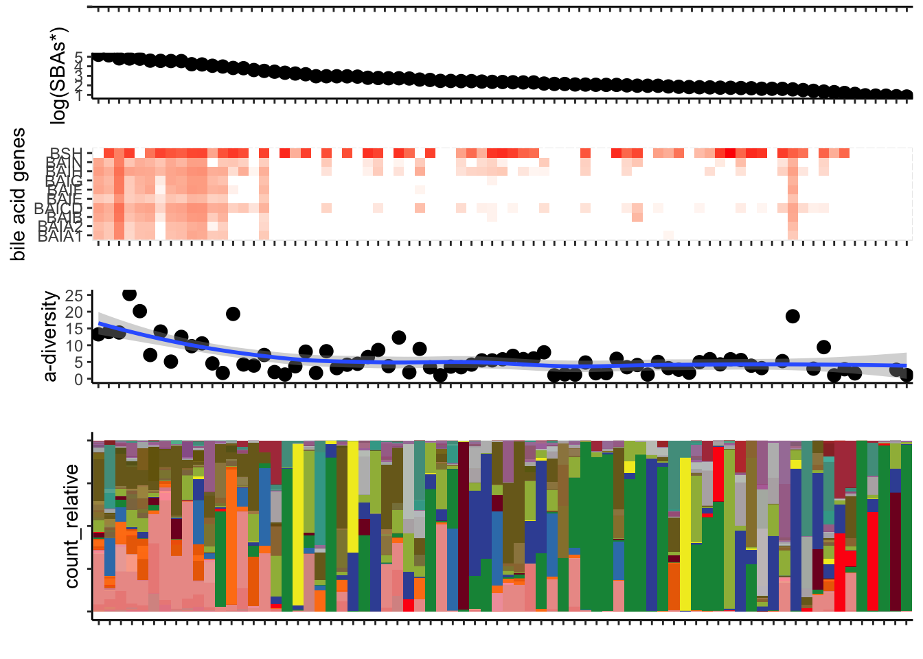
Chapter 7 Create landscape of all peri-GVHD-onset samples (figure 5)
7.1 Define sample order from higher nonUDCA secondary BAs to lower
samples_key<-BSH_metalphlan %>% distinct(sampleid) %>%
  left_join(later_pools_final %>% select(sampleid, secondary_nonUDCA)) %>%
  left_join(cohort_BAS) %>%
  filter(later=="Y") %>%
  arrange(desc(secondary_nonUDCA)) %>%
  left_join(ursodiol) %>% filter(ursodiol2=="Y")

level_order <- samples_key$sampleid
7.2 GI GVHD plot
gi_gvhd_plot<-cohort_BAS %>%
  filter(later=="Y") %>%
  ggplot((aes(x = factor(sampleid, levels = level_order), y = 1, fill = GI_GVHD))) +
  geom_raster(color = "black", size = 0.5) +
  theme_classic()+ theme(axis.text.x=element_blank())+
  xlab("")+
  ylab("")+
  scale_fill_manual(values=c("white", "dodgerblue4"))+
  theme(axis.text.y = element_blank())+
  theme(legend.position = "none") #only for plotting reasons

gi_gvhd_plot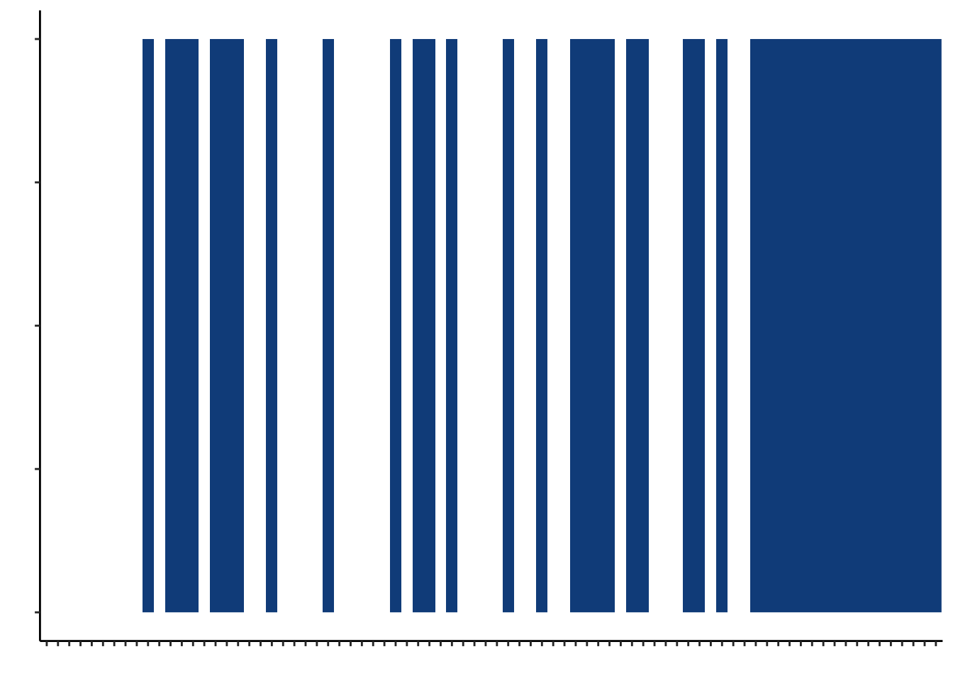
7.3 SBA plot
sba_plot<-ggplot(samples_key, aes(x=factor(sampleid, level=level_order), y=log10(secondary_nonUDCA)))+
  geom_point(size=3)+theme_classic()+
  ylab("log(SBAs*)")+
  theme(axis.text.x=element_blank())+
  xlab("")
sba_plot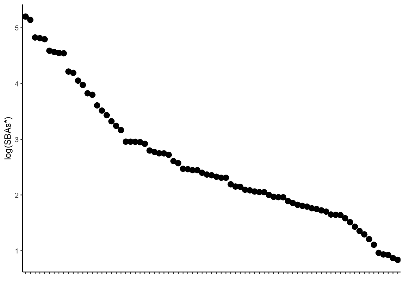
7.4 A-diversity plot
adiv_pre<-cohort_BAS %>%
  filter(later=="Y") %>%
  left_join(asv_alpha_all) %>%  #add a-diversity
  inner_join(samples_key) %>%
  arrange(desc(secondary_nonUDCA)) %>%
          mutate(rank = 1:nrow(.))

adiv_plot<-ggplot(adiv_pre, aes(x = rank, y = simpson_reciprocal)) +
  geom_point(size=3) +
  geom_smooth(method = "loess") +
  theme_classic() +
  ylab("a-diversity") +
  #xlab("sampleid") +
  theme(axis.text.x = element_blank()) +
  xlab("") +
  scale_x_discrete(limits = adiv_pre$rank[order(-adiv_pre$rank)])

adiv_plot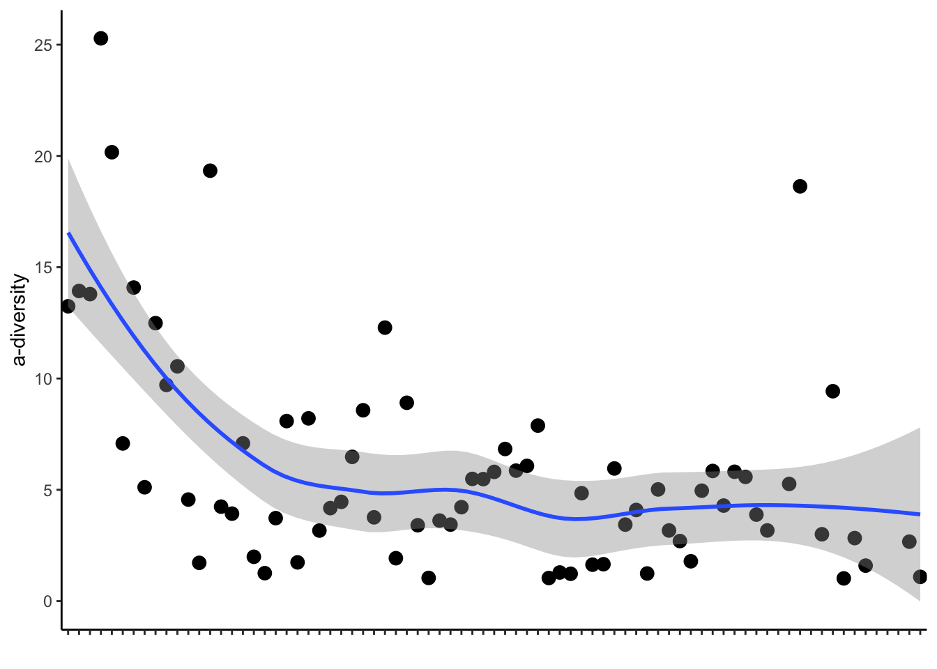
7.5 Bile acid related genes
bai_genes_clean$sampleid <-gsub("FMT_", "FMT.", bai_genes_clean$sampleid)

ba_genes_pre<-samples_key %>%
  select(sampleid, GI_GVHD, secondary_nonUDCA) %>%
  left_join(BSH_metalphlan %>%
              select(sampleid, cpm, KOID)) %>%
  rename(gene=KOID) %>%
  mutate(gene=ifelse(gene=="K01442", "BSH", NA)) %>%
  distinct() %>%
  spread(key=gene, value=cpm, fill=0)

operon_genes_pre<-samples_key %>%
  left_join(bai_genes_clean) %>%
  select(sampleid, cpm, gene) %>%
  distinct() %>%
  spread(key=gene, value=cpm, fill=0)

pre_bai_plot<-ba_genes_pre %>%
  left_join(operon_genes_pre) %>%
  select(-GI_GVHD, -secondary_nonUDCA) %>%
  gather("gene", "cpm", names(.)[2]:names(.)[ncol(.)])


bai_plot<-pre_bai_plot %>%
  ggplot(aes(x=factor(sampleid, level=level_order), y=gene, fill=log10(cpm+0.05)))+
           geom_tile()+
  xlab("")+
  ylab("bile acid genes")+
  scale_fill_gradient(low="white", high="red")+
  theme(axis.text.x=element_blank())+
  theme(legend.position = "none") #only for plotting reasons
bai_plot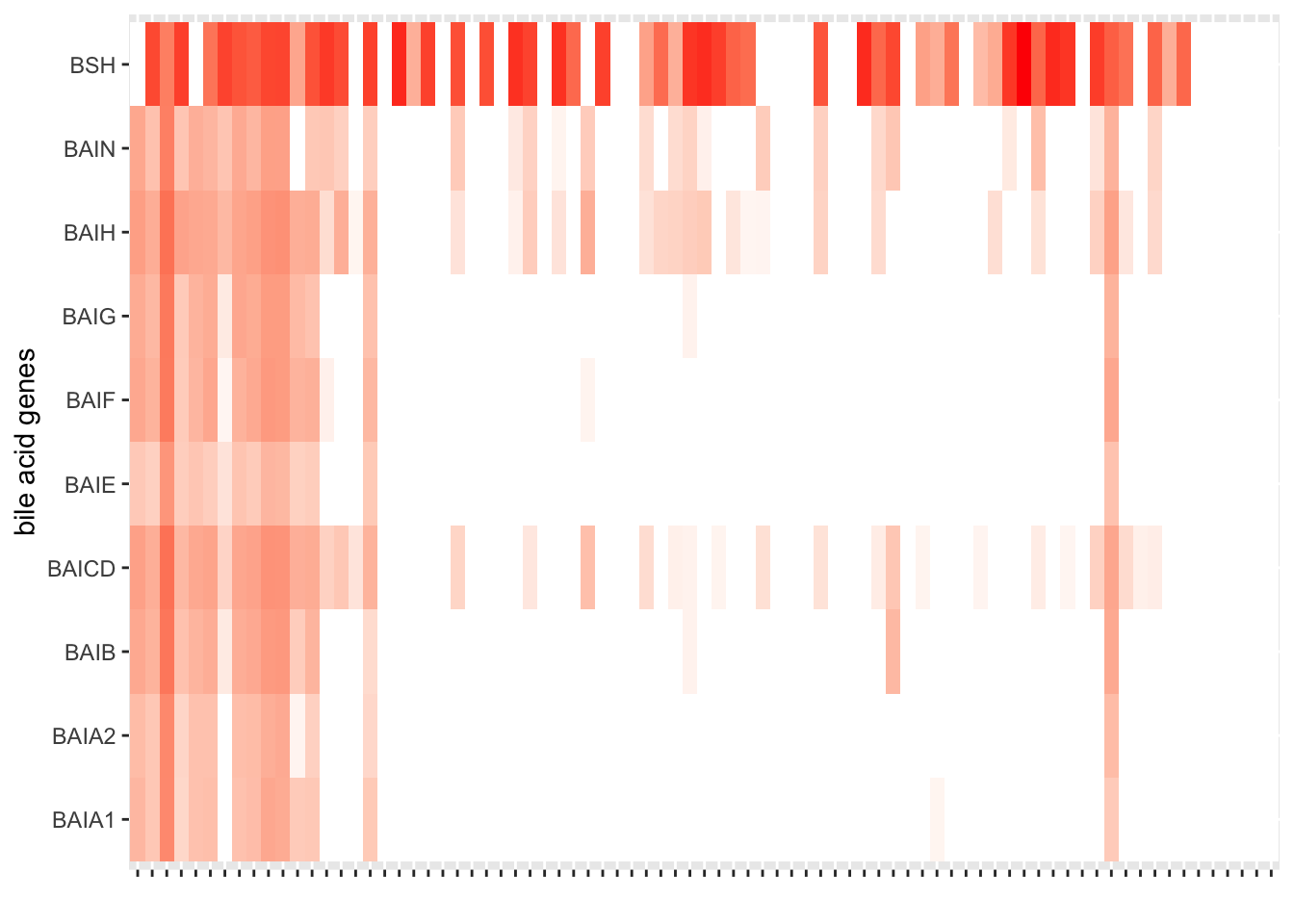
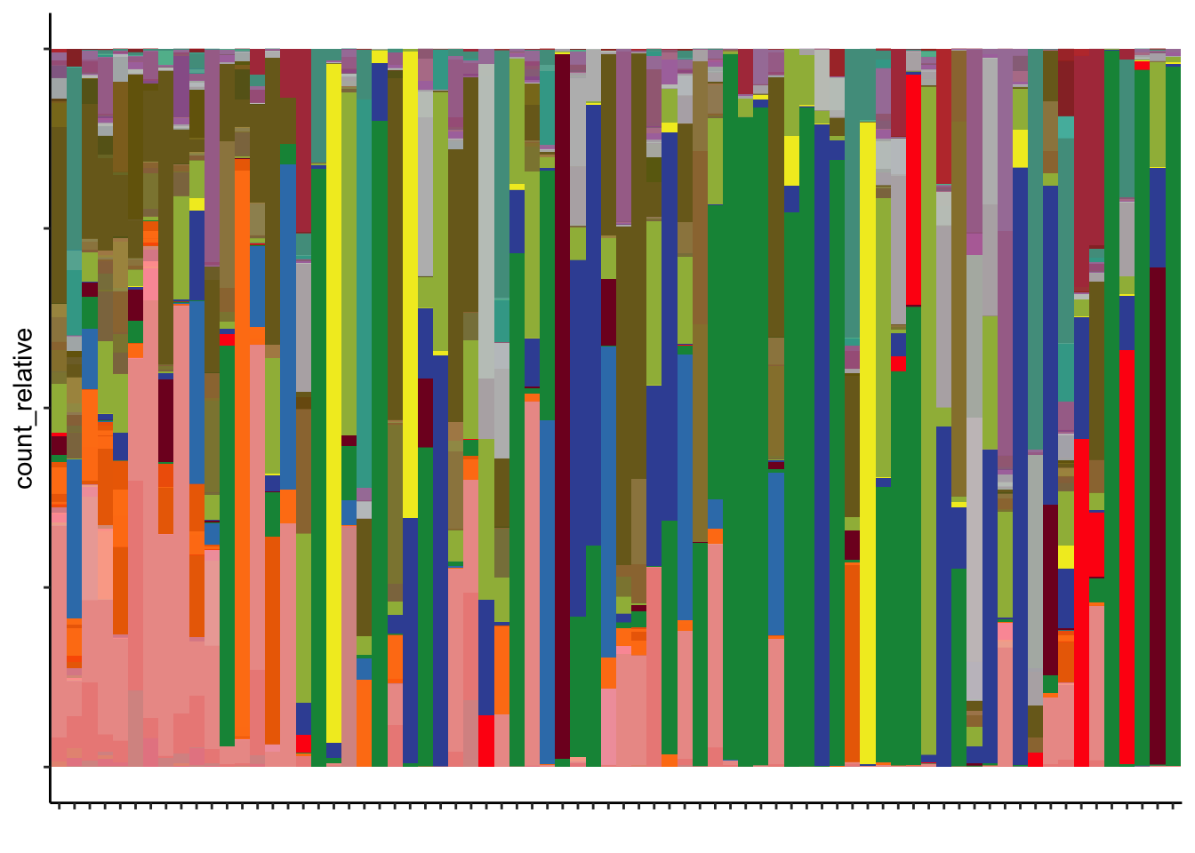
7.6 Microbiome composition
setDT(asv_annotation_blast_color_ag)
asv_color_base_set = unique(asv_annotation_blast_color_ag[,.(color_label_group,color_base)])
color_base_set_asv_carT = asv_color_base_set$color_base
names(color_base_set_asv_carT) =asv_color_base_set$color_label_group;
gg = ggplot(asv_color_base_set, aes(color_label_group,y=1,fill=color_label_group)) + geom_tile()  +
  scale_fill_manual(values = color_base_set_asv_carT) +
  theme_classic() +
  theme(axis.text.x = element_text(angle=60,hjust = 1)) +
  theme(legend.position = "none")

#color_set_asv_carT maps each distinct taxonomic group to its corresponding color.
asv_color_set = unique(asv_annotation_blast_color_ag[,.(color,color_label_group_distinct,color_label_group,color_base)])
color_set_asv_carT = asv_color_set$color
names(color_set_asv_carT) =asv_color_set$color_label_group_distinct;
setDT(counts_samples)
setDT(asv_annotation_blast_color_ag)
m = merge(counts_samples[,.(asv_key,sampleid,
                         count,count_relative,count_total)],
          asv_annotation_blast_color_ag[,.(asv_key,color_label_group_distinct)]);

sample_composition <- m %>%
  left_join(cohort_BAS %>% select(PID, sampleid)) %>%
  left_join(cohort_BAS) %>%
  filter(later=="Y")


m1<-sample_composition %>%
  group_by(sampleid, color_label_group_distinct) %>%
  inner_join(samples_key) %>%
  mutate(sampleid = fct_reorder(sampleid, desc(secondary_nonUDCA)))

m1$color_label_group_distinct = factor(m1$color_label_group_distinct,levels = sort(unique(m1$color_label_group_distinct),decreasing = T));
gg_composition = ggplot(m1,
                        aes(x=factor(sampleid, levels=level_order),
                            y=count_relative,
                            fill=color_label_group_distinct) ) +
  geom_bar(stat = "identity",position="fill",width = 1) +
  theme_classic() +
  theme(axis.text.x = element_blank(),
        axis.text.y = element_blank(),
        legend.position = "none") +
  xlab("")+
  scale_fill_manual(values = color_set_asv_carT);
print(gg_composition)